DBSCAN: What, Why, and How?
As a school exercise, I was tasked with studying a data science algorithm, implementing it myself, and explaining how it worked. I chose to look into DBSCAN since I wasn’t familiar with it before. So today I’ll be explaining what it is, why you might use it, and how it works.
What is it?
Put simply, DBSCAN is a clustering algorithm. It is a form of unsupervised machine learning, where you give it a collection of data and it finds groups of data points that are similar to each other (the clusters). “Unsupervised” in machine learning means it finds patterns in the data on its own. You do not have to tell it how many clusters there are, it simply finds them.
DBSCAN’s full name is Density Based Spatial Clustering of Applications with Noise. It was first proposed by mathematicians in 1996, and is still widely used today.
Why should we use it?
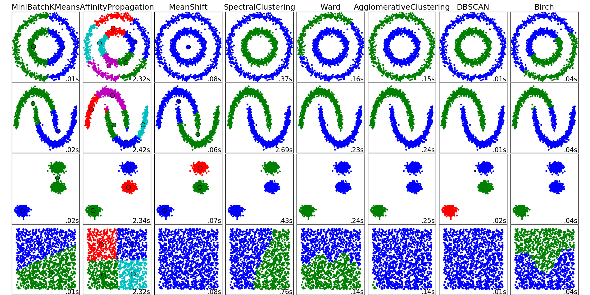
Different clustering algorithms are better for different situations. DBSCAN’s strengths are that it can handle clusters of any shape and any number of clusters, it handles outliers well, and it requires only two parameters. This means it is simpler to set up than many other algorithms, and can work on a variety of data.
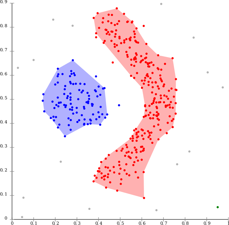
For example, the graph below could not be correctly clustered using some other algorithms like K-Means. Image source
One place where DBSCAN is used commercially is in recommendation engines. You can use it to discover “clusters” of users based on the products they buy, or shows they watch. For example, if you watch a lot of Breaking Bad shows, Netflix could use a clustering algorithm to find other users who watch similar shows, and recommend some of those shows to you. (Netflix likely uses a variety of methods for this, clustering is just one possibility)
DBSCAN is not perfect, of course. If it were then why would we even have other algorithms? It cannot separate clusters when they overlap, and it can have a hard time with clusters of varying densities. Also, those two parameters it requires can also be a disadvantage, since they must be set appropriately for DBSCAN to give good results. There are many clustering algorithms, so determining which one to use is often an important first step.
How does it work?
I mentioned two parameters that DBSCAN requires, those are ε (epsilon) and minPts. ε is the maximum distance two points can be from each other to be considered neighbors, and minPts is the minimum number of points there must be in a neighborhood for it to be considered a cluster.
DBSCAN has three definitions of points:
- A point is a core point if at least minPts points are within distance ε of it, including itself.
- A point is a border point if it is within ε distance of a core point, but has fewer than minPts points around it.
- Any point that is not within ε distance of a core point is an outlier, or noise.
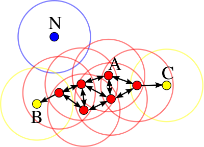
A cluster includes all connected core and border points. In the example below, all red points are the core points of a cluster, while B and C are border points in that cluster. Point N is an outlier. Image source
Using those definitions of points and clusters, it is relatively simple to implement the actual DBSCAN algorithm. For each point, find all neighbors within distance ε. If there are too few neighbors, the point is marked as an outlier and we move on. If there are enough neighbors, we then start checking the neighbors of those neighbors, until all points in that cluster have been found.
Since we can check if a point has already been found this way at the beginning of the loop, it is only necessary to check the neighbors of each point once. This makes the runtime complexity of DBSCAN O(n2).
While different implementations of DBSCAN will usually get the exact same results on a given data set, it is not entirely deterministic. If a border point is within range of two or more clusters, the order in which points are traversed will determine which cluster that point is assigned to.
Implementing it
As I mentioned at the beginning, I also wrote my own implementation of this. In practice, this will almost certainly be unnecessary since there are many freely available implementations. I compared mine to Scikit-Learn’s version, since I was also using Python.
There are several fancy ways you can optimize this function, such as using a database index or a K-D Tree, either of which can significantly speed up finding neighbors of a given point.
I kept things fairly simple, first I just wrote my own O(n) function that checked the distance of all other points to one point and returned the neighbors that were close enough. Later I worked in the SciPy function pdist which sped that up a little.
The rest of the algorithm does pretty much what I described in the section above. For each point, if it hasn’t already been found, check it’s neighbors. If there are enough, start checking the neighbors of those points to find each cluster.
And the results are exactly the same as SKlearn’s version:
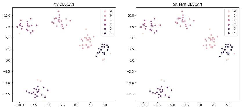
Though, predictably, my own version runs slower. With n=100, my implementation took 30ms while SKlearn took only 6ms. And a second trial with n=250 ran in 126ms vs 4ms. That just goes back to my earlier statement, there’s usually no reason to write your own implementation if a library has already done it. But my goal here was to achieve the same output, which I did achieve.
If you would like to see the code itself, here’s the Python notebook on Google colab.